【Streamlit】粒子法シミュレーション

JS2IIU

8か月前

こんにちは、JS2IIUです。
本記事では、「粒子法シミュレーション」の基礎からPythonによる実装、さらにStreamlitを活用したリアルタイム可視化までを丁寧に解説していきます。粒子法は物理現象を直感的に表現できる強力な手法ですが、複雑に感じることも多いかもしれません。Streamlitの利用により、シミュレーション結果を手軽にインタラクティブなUIで操作・確認していきます。今回もよろしくお願いします

1. はじめに
1. 粒子法シミュレーションとは？
2. なぜStreamlitを使うのか？
2. 粒子法シミュレーションの基本概念
3. Pythonで作る粒子法シミュレーションの基本実装
4. Streamlitで粒子法シミュレーションをリアルタイム可視化
サンプルコード全体
5. パフォーマンスチューニングのポイント
1. Python高速化テクニック
2. Streamlit上の処理負荷低減
6. 実際の応用例と拡張アイデア
7. まとめと今後の展望
参考資料・学習リソース

1. はじめに

粒子法シミュレーションとは？

粒子法とは、物理系を「粒子の集合」として表現し、粒子の位置や速度を時間的に更新しながら現象を再現する手法です。
特徴的なのは「メッシュ（格子）を使わない」ことです。これは流体や材料の変形など、複雑な形状変化に強いメリットがあります。

代表例として「運動する水滴」「砂の堆積」「群集の移動」など自然現象のモデリングに活用されています。

なぜStreamlitを使うのか？

StreamlitはPythonで簡単にWebアプリを作成できるフレームワークで、複雑なフロントエンドの知識なしにインタラクティブなUIが作成可能です。
シミュレーションのパラメータを動的に変更しながら結果をすぐに確認するには非常に便利な存在です。

では始めていきましょう！

2. 粒子法シミュレーションの基本概念

粒子法の基本原理

粒子：物理量（位置、速度など）を持つ最小単位
粒子の移動：力を受けて粒子は速度や位置を変化させる
相互作用：粒子同士が近接して影響を与え合うことで複雑な挙動が生まれる
力学法則の適用：ニュートン力学の運動方程式に基づく

シミュレーションに必要な要素

粒子の状態（位置、速度、加速度などの属性）
力の計算方法（外力や粒子間力）
時間発展の計算方法（数値積分で状態を更新）

具体例：重力のある粒子系

単純化のため、重力だけが作用する複数の粒子を考えます。
これだけでも粒子の落下や堆積の基本的な動きを表現可能です。

3. Pythonで作る粒子法シミュレーションの基本実装

環境準備

Python3の環境を用意し、以下のライブラリをインストールします。

Python

pip install numpy matplotlib streamlit

pip install numpy matplotlib streamlit

粒子クラスの定義

まず、粒子の属性を管理するクラスを作ります。

Python

import numpy as np

class Particle:
    def __init__(self, position, velocity):
        """
        position: numpy配列（x, y）
        velocity: numpy配列（vx, vy）
        """
        self.position = np.array(position, dtype=float)
        self.velocity = np.array(velocity, dtype=float)
        self.acceleration = np.zeros(2)

import numpy as np

class Particle:
    def __init__(self, position, velocity):
        """
        position: numpy配列（x, y）
        velocity: numpy配列（vx, vy）
        """
        self.position = np.array(position, dtype=float)
        self.velocity = np.array(velocity, dtype=float)
        self.acceleration = np.zeros(2)

力の計算例（重力）

粒子にかかる加速度を重力として設定します。

Python

def apply_gravity(particles, g=np.array([0, -9.81])):
    for p in particles:
        p.acceleration = g  # 重力加速度を設定

def apply_gravity(particles, g=np.array([0, -9.81])):
    for p in particles:
        p.acceleration = g  # 重力加速度を設定

時間発展（Euler法）

位置と速度を単純なオイラー法で更新します。

Python

def update_particles(particles, dt):
    for p in particles:
        p.velocity += p.acceleration * dt
        p.position += p.velocity * dt

def update_particles(particles, dt):
    for p in particles:
        p.velocity += p.acceleration * dt
        p.position += p.velocity * dt

サンプルコード全体例

すでに説明したコードも含めたコード全体です。

Python

import matplotlib.pyplot as plt
import numpy as np


class Particle:
    def __init__(self, position, velocity):
        """
        position: numpy配列（x, y）
        velocity: numpy配列（vx, vy）
        """
        self.position = np.array(position, dtype=float)
        self.velocity = np.array(velocity, dtype=float)
        self.acceleration = np.zeros(2)


def apply_gravity(particles, g=np.array([0, -9.81])):
    for p in particles:
        p.acceleration = g  # 重力加速度を設定

def update_particles(particles, dt):
    for p in particles:
        p.velocity += p.acceleration * dt
        p.position += p.velocity * dt

def simulate(particles, steps=100, dt=0.01):
    positions = []

    for _ in range(steps):
        apply_gravity(particles)
        update_particles(particles, dt)
        positions.append([p.position.copy() for p in particles])

    return positions

# 初期化
particles = [
    Particle(position=[0, 0], velocity=[1, 5]),
    Particle(position=[1, 2], velocity=[-0.5, 3])
]

positions = simulate(particles)

# 最後の位置をプロット
x_vals = [p.position[0] for p in particles]
y_vals = [p.position[1] for p in particles]

plt.scatter(x_vals, y_vals)
plt.xlabel('x')
plt.ylabel('y')
plt.title('Particle Positions After Simulation')
plt.grid(True)
plt.show()

import matplotlib.pyplot as plt
import numpy as np


class Particle:
    def __init__(self, position, velocity):
        """
        position: numpy配列（x, y）
        velocity: numpy配列（vx, vy）
        """
        self.position = np.array(position, dtype=float)
        self.velocity = np.array(velocity, dtype=float)
        self.acceleration = np.zeros(2)


def apply_gravity(particles, g=np.array([0, -9.81])):
    for p in particles:
        p.acceleration = g  # 重力加速度を設定

def update_particles(particles, dt):
    for p in particles:
        p.velocity += p.acceleration * dt
        p.position += p.velocity * dt

def simulate(particles, steps=100, dt=0.01):
    positions = []

    for _ in range(steps):
        apply_gravity(particles)
        update_particles(particles, dt)
        positions.append([p.position.copy() for p in particles])

    return positions

# 初期化
particles = [
    Particle(position=[0, 0], velocity=[1, 5]),
    Particle(position=[1, 2], velocity=[-0.5, 3])
]

positions = simulate(particles)

# 最後の位置をプロット
x_vals = [p.position[0] for p in particles]
y_vals = [p.position[1] for p in particles]

plt.scatter(x_vals, y_vals)
plt.xlabel('x')
plt.ylabel('y')
plt.title('Particle Positions After Simulation')
plt.grid(True)
plt.show()

サンプルコード解説

ライブラリのインポート

Python

import matplotlib.pyplot as plt
import numpy as np

import matplotlib.pyplot as plt
import numpy as np

matplotlib.pyplot はグラフ描画用のライブラリ。
numpy は数値計算ライブラリ。ベクトル・行列計算を行うために使用。

クラス定義：Particle

Python

class Particle:
    def __init__(self, position, velocity):
        self.position = np.array(position, dtype=float)
        self.velocity = np.array(velocity, dtype=float)
        self.acceleration = np.zeros(2)

class Particle:
    def __init__(self, position, velocity):
        self.position = np.array(position, dtype=float)
        self.velocity = np.array(velocity, dtype=float)
        self.acceleration = np.zeros(2)

Particle クラスは1つの粒子の状態（位置・速度・加速度）を表す。
position: 現在の位置（例：[x, y]）
velocity: 現在の速度（例：[vx, vy]）
acceleration: 加速度（最初は0ベクトル）

関数：重力を適用する apply_gravity

Python

def apply_gravity(particles, g=np.array([0, -9.81])):
    for p in particles:
        p.acceleration = g

def apply_gravity(particles, g=np.array([0, -9.81])):
    for p in particles:
        p.acceleration = g

各粒子に重力加速度（デフォルトは地球上の重力 [0, -9.81] m/s²）を設定。
加速度は1ステップごとに更新される。

関数：粒子を1ステップ分更新 update_particles

Python

def update_particles(particles, dt):
    for p in particles:
        p.velocity += p.acceleration * dt
        p.position += p.velocity * dt

def update_particles(particles, dt):
    for p in particles:
        p.velocity += p.acceleration * dt
        p.position += p.velocity * dt

オイラー法を用いて粒子の速度と位置を更新。
dt は時間刻み（例えば 0.01 秒）。

関数：全体のシミュレーション simulate

Python

def simulate(particles, steps=100, dt=0.01):
    positions = []

    for _ in range(steps):
        apply_gravity(particles)
        update_particles(particles, dt)
        positions.append([p.position.copy() for p in particles])

    return positions

def simulate(particles, steps=100, dt=0.01):
    positions = []

    for _ in range(steps):
        apply_gravity(particles)
        update_particles(particles, dt)
        positions.append([p.position.copy() for p in particles])

    return positions

steps: シミュレーションのステップ数（時間の区切り）。
毎ステップごとに重力を適用し、状態を更新。
各ステップごとの位置情報を positions に保存（可視化などに利用可能）。

初期状態の設定とシミュレーションの実行

Python

particles = [
    Particle(position=[0, 0], velocity=[1, 5]),
    Particle(position=[1, 2], velocity=[-0.5, 3])
]

positions = simulate(particles)

particles = [
    Particle(position=[0, 0], velocity=[1, 5]),
    Particle(position=[1, 2], velocity=[-0.5, 3])
]

positions = simulate(particles)

2つの粒子を初期化。
1つ目: 原点から右上へ移動
2つ目: 少し右上に位置し、左上に移動
それらの粒子の運動を simulate() で計算。

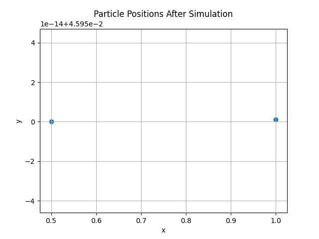
最終状態の可視化

Python

x_vals = [p.position[0] for p in particles]
y_vals = [p.position[1] for p in particles]

plt.scatter(x_vals, y_vals)
plt.xlabel('x')
plt.ylabel('y')
plt.title('Particle Positions After Simulation')
plt.grid(True)
plt.show()

x_vals = [p.position[0] for p in particles]
y_vals = [p.position[1] for p in particles]

plt.scatter(x_vals, y_vals)
plt.xlabel('x')
plt.ylabel('y')
plt.title('Particle Positions After Simulation')
plt.grid(True)
plt.show()

シミュレーション終了時点の各粒子の x 座標・y 座標を取り出し、散布図として描画。

補足：物理シミュレーションのポイント

このコードは基本的な数値シミュレーション（Euler法）を使って運動をモデル化しています。
摩擦や空気抵抗などは考慮しておらず、純粋に重力のみの単純な物理モデルです。
実際には時間刻み dt を小さくすると、より精度の高いシミュレーションが可能になります。

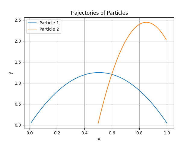
動作イメージ

粒子の軌跡をプロットするようにコードを変更します。

Python

import matplotlib.pyplot as plt
import numpy as np


class Particle:
    def __init__(self, position, velocity):
        self.position = np.array(position, dtype=float)
        self.velocity = np.array(velocity, dtype=float)
        self.acceleration = np.zeros(2)


def apply_gravity(particles, g=np.array([0, -9.81])):
    for p in particles:
        p.acceleration = g


def update_particles(particles, dt):
    for p in particles:
        p.velocity += p.acceleration * dt
        p.position += p.velocity * dt


def simulate(particles, steps=100, dt=0.01):
    positions = []

    for _ in range(steps):
        apply_gravity(particles)
        update_particles(particles, dt)
        positions.append([p.position.copy() for p in particles])

    return positions


# 初期化
particles = [
    Particle(position=[0, 0], velocity=[1, 5]),
    Particle(position=[1, 2], velocity=[-0.5, 3])
]

# シミュレーション実行
positions = simulate(particles)

# 粒子ごとに軌跡を抽出して描画
num_particles = len(particles)
steps = len(positions)

for i in range(num_particles):
    x_vals = [positions[step][i][0] for step in range(steps)]
    y_vals = [positions[step][i][1] for step in range(steps)]
    plt.plot(x_vals, y_vals, label=f'Particle {i+1}')

plt.xlabel('x')
plt.ylabel('y')
plt.title('Trajectories of Particles')
plt.legend()
plt.grid(True)
plt.show()

import matplotlib.pyplot as plt
import numpy as np


class Particle:
    def __init__(self, position, velocity):
        self.position = np.array(position, dtype=float)
        self.velocity = np.array(velocity, dtype=float)
        self.acceleration = np.zeros(2)


def apply_gravity(particles, g=np.array([0, -9.81])):
    for p in particles:
        p.acceleration = g


def update_particles(particles, dt):
    for p in particles:
        p.velocity += p.acceleration * dt
        p.position += p.velocity * dt


def simulate(particles, steps=100, dt=0.01):
    positions = []

    for _ in range(steps):
        apply_gravity(particles)
        update_particles(particles, dt)
        positions.append([p.position.copy() for p in particles])

    return positions


# 初期化
particles = [
    Particle(position=[0, 0], velocity=[1, 5]),
    Particle(position=[1, 2], velocity=[-0.5, 3])
]

# シミュレーション実行
positions = simulate(particles)

# 粒子ごとに軌跡を抽出して描画
num_particles = len(particles)
steps = len(positions)

for i in range(num_particles):
    x_vals = [positions[step][i][0] for step in range(steps)]
    y_vals = [positions[step][i][1] for step in range(steps)]
    plt.plot(x_vals, y_vals, label=f'Particle {i+1}')

plt.xlabel('x')
plt.ylabel('y')
plt.title('Trajectories of Particles')
plt.legend()
plt.grid(True)
plt.show()

粒子が放物線を描いて落下する様子が確認できます。

4. Streamlitで粒子法シミュレーションをリアルタイム可視化

Streamlit基本的なUI作成例

パラメータ調整用のスライダーやボタンを追加します。

Python

import streamlit as st

num_particles = st.slider('粒子数', 1, 50, 10)
gravity_strength = st.slider('重力加速度', 0.0, 20.0, 9.81)
start_button = st.button('シミュレーション開始')

import streamlit as st

num_particles = st.slider('粒子数', 1, 50, 10)
gravity_strength = st.slider('重力加速度', 0.0, 20.0, 9.81)
start_button = st.button('シミュレーション開始')

シミュレーション結果の描画

matplotlibをStreamlitに埋め込みます。

Python

import io

fig, ax = plt.subplots()

# 仮の粒子位置
x = np.random.rand(num_particles)
y = np.random.rand(num_particles)

ax.scatter(x, y)
ax.set_xlim(-10, 10)
ax.set_ylim(-10, 10)

buf = io.BytesIO()
fig.savefig(buf, format="png")
st.image(buf)

import io

fig, ax = plt.subplots()

# 仮の粒子位置
x = np.random.rand(num_particles)
y = np.random.rand(num_particles)

ax.scatter(x, y)
ax.set_xlim(-10, 10)
ax.set_ylim(-10, 10)

buf = io.BytesIO()
fig.savefig(buf, format="png")
st.image(buf)

粒子位置のリアルタイム更新（簡易例）

Python

import time

particles = [Particle(position=[0, i], velocity=[0, 0]) for i in range(num_particles)]

if start_button:
    for _ in range(100):
        apply_gravity(particles, g=np.array([0, -gravity_strength]))


     update_particles(particles, dt=0.05)

        fig, ax = plt.subplots()
        x_vals = [p.position[0] for p in particles]
        y_vals = [p.position[1] for p in particles]

        ax.scatter(x_vals, y_vals)
        ax.set_xlim(-10, 10)
        ax.set_ylim(-10, 10)

        st.pyplot(fig)
        time.sleep(0.05)

import time

particles = [Particle(position=[0, i], velocity=[0, 0]) for i in range(num_particles)]

if start_button:
    for _ in range(100):
        apply_gravity(particles, g=np.array([0, -gravity_strength]))


     update_particles(particles, dt=0.05)

        fig, ax = plt.subplots()
        x_vals = [p.position[0] for p in particles]
        y_vals = [p.position[1] for p in particles]

        ax.scatter(x_vals, y_vals)
        ax.set_xlim(-10, 10)
        ax.set_ylim(-10, 10)

        st.pyplot(fig)
        time.sleep(0.05)

上記はシンプルな例ですが、Streamlitのst.pyplot()をループ内で更新して粒子の動きをリアルタイムに表示できます。

サンプルコード全体

Streamlitを使って可視化アプリにしました。設定関連はサイドバーに設置して全体が見やすいUIにしています。

Python

import streamlit as st
import numpy as np
import matplotlib.pyplot as plt
import time
import io

# 粒子クラス定義
class Particle:
    def __init__(self, position, velocity):
        self.position = np.array(position, dtype=float)
        self.velocity = np.array(velocity, dtype=float)
        self.acceleration = np.zeros(2)

# 重力適用関数
def apply_gravity(particles, g):
    for p in particles:
        p.acceleration = g

# 粒子位置更新関数（オイラー法）
def update_particles(particles, dt):
    for p in particles:
        p.velocity += p.acceleration * dt
        p.position += p.velocity * dt

# Streamlit UI
st.title("粒子法シミュレーション")

# サイドバーに設定項目を追加
st.sidebar.header("シミュレーション設定")
num_particles = st.sidebar.number_input("粒子数", min_value=1, max_value=10000, value=100)
gravity_strength = st.sidebar.number_input("重力加速度 (m/s²)", min_value=0.0, max_value=100.0, value=9.8)
dt = st.sidebar.number_input("時間刻み (dt)", min_value=0.0001, max_value=1.0, value=0.01, format="%.4f")
steps = st.sidebar.number_input("ステップ数", min_value=1, max_value=100000, value=1000)
start_sim = st.sidebar.button("シミュレーション開始")

# シミュレーションの実行
if start_sim:
    st.success("シミュレーションを開始します。")

    # 粒子をランダムな初期位置・速度で初期化
    particles = [
        Particle(position=[np.random.uniform(-5, 5), np.random.uniform(0, 5)],
                 velocity=[np.random.uniform(-1, 1), np.random.uniform(2, 5)])
        for _ in range(num_particles)
    ]

    # 表示エリアの初期化
    plot_area = st.empty()

    for step in range(steps):
        apply_gravity(particles, g=np.array([0, -gravity_strength]))
        update_particles(particles, dt)

        # 描画
        fig, ax = plt.subplots()
        x_vals = [p.position[0] for p in particles]
        y_vals = [p.position[1] for p in particles]

        ax.scatter(x_vals, y_vals, c='blue')
        ax.set_xlim(-10, 10)
        ax.set_ylim(-10, 10)
        ax.set_title(f"Step {step + 1}")
        ax.set_xlabel("x")
        ax.set_ylabel("y")
        ax.grid(True)

        plot_area.pyplot(fig)
        plt.close(fig)
        time.sleep(0.03)

import streamlit as st
import numpy as np
import matplotlib.pyplot as plt
import time
import io

# 粒子クラス定義
class Particle:
    def __init__(self, position, velocity):
        self.position = np.array(position, dtype=float)
        self.velocity = np.array(velocity, dtype=float)
        self.acceleration = np.zeros(2)

# 重力適用関数
def apply_gravity(particles, g):
    for p in particles:
        p.acceleration = g

# 粒子位置更新関数（オイラー法）
def update_particles(particles, dt):
    for p in particles:
        p.velocity += p.acceleration * dt
        p.position += p.velocity * dt

# Streamlit UI
st.title("粒子法シミュレーション")

# サイドバーに設定項目を追加
st.sidebar.header("シミュレーション設定")
num_particles = st.sidebar.number_input("粒子数", min_value=1, max_value=10000, value=100)
gravity_strength = st.sidebar.number_input("重力加速度 (m/s²)", min_value=0.0, max_value=100.0, value=9.8)
dt = st.sidebar.number_input("時間刻み (dt)", min_value=0.0001, max_value=1.0, value=0.01, format="%.4f")
steps = st.sidebar.number_input("ステップ数", min_value=1, max_value=100000, value=1000)
start_sim = st.sidebar.button("シミュレーション開始")

# シミュレーションの実行
if start_sim:
    st.success("シミュレーションを開始します。")

    # 粒子をランダムな初期位置・速度で初期化
    particles = [
        Particle(position=[np.random.uniform(-5, 5), np.random.uniform(0, 5)],
                 velocity=[np.random.uniform(-1, 1), np.random.uniform(2, 5)])
        for _ in range(num_particles)
    ]

    # 表示エリアの初期化
    plot_area = st.empty()

    for step in range(steps):
        apply_gravity(particles, g=np.array([0, -gravity_strength]))
        update_particles(particles, dt)

        # 描画
        fig, ax = plt.subplots()
        x_vals = [p.position[0] for p in particles]
        y_vals = [p.position[1] for p in particles]

        ax.scatter(x_vals, y_vals, c='blue')
        ax.set_xlim(-10, 10)
        ax.set_ylim(-10, 10)
        ax.set_title(f"Step {step + 1}")
        ax.set_xlabel("x")
        ax.set_ylabel("y")
        ax.grid(True)

        plot_area.pyplot(fig)
        plt.close(fig)
        time.sleep(0.03)

5. パフォーマンスチューニングのポイント

Python高速化テクニック

NumPyによるベクトル化
粒子の位置・速度を配列で扱い、ループを減らす
JITコンパイル（Numba）
関数にデコレーターを付けて高速化可能

Streamlit上の処理負荷低減

@st.cacheの利用
変化しない処理結果の再計算を防ぐ
計算頻度の調整
必要なタイミングだけ計算を行う

6. 実際の応用例と拡張アイデア

粒子法のプログラムを発展させるためのキーワードを列挙します。

粒子法活躍分野例

流体シミュレーション（SPH法など）
材料変形シミュレーション
群集や群れの動きのモデリング

コード拡張例

粘性や摩擦を加える
粒子間のばね力を導入
3D空間での拡張

他技術との連携

機械学習モデルによるパラメータ推定
Plotly/Dashによる高度な可視化
GPU対応（CuPyやPyCUDA）

7. まとめと今後の展望

本記事では、粒子法シミュレーションの基礎理論からPythonでの実装、そしてStreamlitを使ったリアルタイム可視化まで説明しました。
Streamlitならではの手軽にインタラクティブなUI作成が、物理モデリングの学習やデモに最適です。将来的にはOpenMPやGPUを使った大規模シミュレーションへのチャレンジも視野に入れてみてください。

参考資料・学習リソース

最後までお読みいただきありがとうございました。